2 Cherenkov ring reconstruction

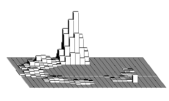
A typical RICH detector consists of a two-dimensional array (grid) of several thousand photosensitive cells (pads). During an event a number of Cherenkov photons produced by a detected particle fall on the pads and form a ring (or ellipse). In fact, each photon, while registered by the RICH, produces signals in a cluster of adjacent pads near the pad that it hits, see Fig. 1. Thus in order to implement the idea of using the raw data directly, one should fit a ring to a few pad clusters, each cluster corresponds to one photon in the ring. This picture sharply contrasts with traditional fitting models based on the random and independent deviations of measured points from the circle to be fitted. In our approach, the cells are fixed but the energy measurements (amplitudes) have random character.
In order to simplify the problem many traditional methods start with a time-consuming calculation of the hit centers of photons from the raw data. However, during this hit-extracting procedure one loses the detailed information of individual pad amplitudes contained in the raw data. Besides, these procedures are, as usual, inaccurate in the cases of close, overlapping clusters.
 

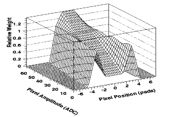
Figure 1: 3D images of simulated discretized signals of one Cherenkov ring	Figure 2: bihorn 2D weight function piecewise linearly approximated

Therefore the idea of ring fitting directly from the raw data can potentially result in faster and more accurate algorithms. In addition, two important features of RICH detectors must be taken into account: (i) the energy measured in the pads is discretized and signals both too small and too large are cut off; (ii) the high occupancy of RICH detectors - the abundance of background noise and possible presence of two or more overlapping rings. These RICH data features considerably violate the crucial assumptions of normality and independence of errors on which the classical least square fit (LSF) is based. It is assumed that measured point deviations from the observed ring are normally distributed independent variables with the common probability density function (p.d.f.) 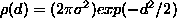 . However, these violations often cause a complete breakdown of the LSF, since data are contaminated by background measurements with p.d.f. u(d) and, therefore 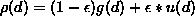 , where  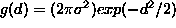and  is the background rate. In such cases the robust weighted least square procedure 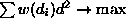 works better. The optimal weight function w(d) for the uniform background distribution u(d) = const was derived in our earlier papers [4, 6]

w(x) = s^-2 1 +

The main problem is to take into account such an essential information as signal amplitudes measured in each pad.
Corresponding formulae for the optimal weight functions have been derived in ref. [6] by the maximum likelihood approach. The formula was obtained for a more general track-finding problem, when a track passing through a detector hits one of many parallel coordinate planes (pad rows). Each hit results in energy deposition in neighboring pads. The total amount of the released energy, E, is a random variable with some p.d.f. f(E),  . The spatial distribution of the deposited energy among pads is bell-shaped, say, a Gaussian, centered at the actual hit point a with a constant variance  . The calculation gave

w(d;A) =                                        (1)

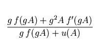
 where 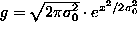 , u(A) is p.d.f. of a background amplitude A measured in the given pad.
If the distribution f(E) is specified as an exponential one with the mean  , i.e.  , then for a wide choice of the background component u(d) (uniform or Gaussian with a wide  or even an exponential one with a large mean value in the cases of  -electrons) we obtain quite an interesting 2D-weight ``surface'', see Fig. 2. For weak signals with a small amplitude A the weight as a function of the distance d has a ``bi-horn'' shape with two pronounced peaks merging together when A is growing. In a track-finding problem, this bimodal weight function is quite natural, it indicates that weaker signals are less likely to appear in the closest vicinity of the track line. Stronger signals are most likely to appear right on the track line, hence the weight function has a narrow single peak. Another problem appears in some experiments when in a certain pad row all the signals are very weak. They will be all rejected by the bimodal weight function, even though within that row the signals may have a nice bell-shaped distribution with a local peak right on the track. In this case one can apply a prior normalization of signals in each pad row in a narrow corridor around the expected track line, see [7]. Lastly, in track-finding applications of bimodal weights to STAR TPC data, we approximated nonlinear optimal weights by simple piece-wise linear functions [7] (see fig. 2).
However, direct application of (1) to the circle fitting using the pad raw data runs into two obstacles: (i) it is very likely that some pads with a small amplitude appear right on the fitted circle, see Fig. 1; (ii) the substantial variability of photon energies distributed according to f(x). Both problems are solved in ref. [6] by ``integrating away'' hidden parameters. The optimal weights have bimodal shape, but their efficiency is lower due to disregarding some weak signals in areas between clusters. One more circle fitting problem relates to the frequent case of several crossing circles. If one would fit them one by one, an extra data contamination appears due to the influence of points of the ``stranger'' circle in the crossing area. So it would be more reasonable to fit those circles simultaneously. For solving the problem of simultaneous fitting of two or more circles it is necessary to create a single equation for several circles. This is done in a way generalizing [8] by multiplying the corresponding circle equations. The LSF estimation of all parameters requires the search for the global minimum of the non-linear functional  , where for two circles. A linearization of L is done similarly to ref. [4]. Details can be found in ref. [9].

We tested the bimodal weight function in a numerical experiment and compared it against two unimodal weights: Huber's [10], Tukey's [11] and the constant one  for the classical LSF. Results for the single circle experiment are summarized in the table 1. All rms values are given in bin-size, the half-width of the signal shape is also equal to bin-size (  ). The noise distribution is uniform with signal/noise ratio = 1.

 

method	Pf	rmsa, b	rmsR
LSF	0.7570	0.231	0.420
Huber	0.1702	0.252	0.321
Tukey (c = 4)	0.0415	0.232	0.144
Tukey (c = 3)	0.0821	0.240	0.157
bimodal	0.0513	0.219	0.130

Table 1. Numerical characteristics of three algorithms for circle fitting to simulated data. Here P_f is the probability of a complete failure, when a and b are off more than one bin size.

Only Tukey's unimodal biweight with c=4 stands the competition with our bimodal one. The numerical results for two circles are shown in the table 2. Simulation details can be found in ref. [9].

 

distance	Pf	rmsa, b	rmsc, d
1	0.0701	0.429	0.430
10	0.0474	0.333	0.390

Table 2. Numerical characteristics for two circles fitting to simulated data using bimodal weights. Distances are given in bin-size

Besides to be as close to real raw data as possible, a GEANT simulation was made of pad structure for Cherenkov rings. We superimposed them into the real background of the CERES Pb-AU'95 RICH data. Results of the ring radius accuracy were comparable (not worse) than those presented in ref. [4].

1999-01-24